Strawfish Pre Lab
We put twenty blue and twenty yellow straws into a paper bag to represent alleles in "strawfish" population. The blue and yellow alleles dictate an incomplete dominance. A strawfish is blue when it contains two blue alleles (BB). Also a strawfish is yellow when it contains yellow alleles (YY). However, a straw fish is green when its colors are heterozygous, having one blue and one yellow (BY).
We completed this test to simulate the different natural selection environmental factors. The natural selection factor of test three was the green fish, who were flavorful, causing every other green fish to be eaten by a predator. The first round was a control group where none of the strawfish were eaten.
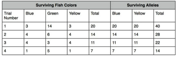
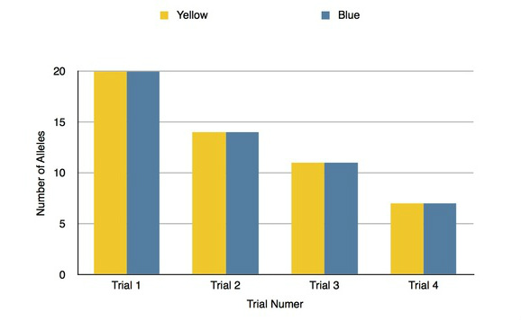
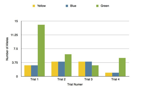
After the first round, we had a high number of green fish and a low number of blue and yellow fish that were equal. In the second trial, we got an equal number of blue and yellow fish again, and also a high number of green fish. After half of the green fish were consumed by preditors, the proportion of the alleles in the population dropped greatly, however the number of yellow and blue alleles stayed equal. During the third round, the blue and yellow fish had the same number and the green fish remained the largest proportion leading to another large loss of alleles. Since the blue and yellow fish were consistently equal, the proportion of surviving alleles remained .5 to .5. For the final trial, the blue and yellow fish were again the same, each only having one. Because there was a large amount of green fish, many of the fish were "eaten" precipitating another significant loss of alleles.
We completed this test to simulate the different natural selection environmental factors. The natural selection factor of test three was the green fish, who were flavorful, causing every other green fish to be eaten by a predator. The first round was a control group where none of the strawfish were eaten.
After the first round, we had a high number of green fish and a low number of blue and yellow fish that were equal. In the second trial, we got an equal number of blue and yellow fish again, and also a high number of green fish. After half of the green fish were consumed by preditors, the proportion of the alleles in the population dropped greatly, however the number of yellow and blue alleles stayed equal. During the third round, the blue and yellow fish had the same number and the green fish remained the largest proportion leading to another large loss of alleles. Since the blue and yellow fish were consistently equal, the proportion of surviving alleles remained .5 to .5. For the final trial, the blue and yellow fish were again the same, each only having one. Because there was a large amount of green fish, many of the fish were "eaten" precipitating another significant loss of alleles.
Charts and Table
Hardy-Weinberg
The Hardy-Weinberg equation gives us the ability to see if a population. The equation is p^2 + 2pq + q^2 = 1. P is the frequency of the dominant allele and q is the frequency of the recessive allele. This equation shows whether or not the population is at Hardy-Weinberg equilibrium. There are find conditions that must be met in order to In order to use the Hardy-Weinberg equation.
No mutations
Random mating
No natural selection that affects the population
Large population
No gene flow
Populations can only reach equilibrium over an extended amount of time because the conditions a rarely met at a single time period.
No mutations
Random mating
No natural selection that affects the population
Large population
No gene flow
Populations can only reach equilibrium over an extended amount of time because the conditions a rarely met at a single time period.
Cases One and Two
Every student in the classroom was provided with two cards. One had an A and the other had an a. These cards represent the gametes of each student. The students then randomly picked partners to mate with. When students mate, they both give one gamete randomly to form their offsprings genetic code. Each student then took the new genotype to use to continue mating with others. This process continued for five generations.
The class had 289 alleles in the first round; 174 alleles of A and 115 alleles of a. The p of the first case is thus .602 and the q is .398. When we put these numbers into the Hardy-Weinberg equation, we got .3624+.4792+.1584=1. The initial class frequency for the first case was AA=.25, Aa=.5, and aa=.25. The final frequencies for the first case were AA=.3624, Aa=.4792, and aa=.1584. These results indicated that the population did evolve, because the genotype proportions changed. There was then a higher proportion of AA and a lower proportion of aa. The first case results differed from the initial frequencies because the class population was too small to gather precise population data for the Hardy-Weinberg equation, skewing the data.
The second case had the same procedure as the first, however the homozygous recessive offspring died, forcing the students to mate until they all have a surviving offspring. The initial class frequency was the same as in the first case: A=.25, Aa=.5, and aa=.25. The ultimate class allele total was 334. There were 220 A alleles and 114 a alleles.The p in the second case was .659 and the q was .341. This made the final class frequencies in the second case AA=.434, Aa=.45, and aa=.116. This displayed as loss of homozygous recessive organisms, but there remained some aa organisms because of the a allele in the heterozygous organisms. The recessive trait would not be eliminated in large populations because the heterozygous members of the population would keep the recessive gene. Our gametes did not match the inition Hardy-Weinburg equation because
Sources of Error
The sources of error in this lab would be certain individuals in the class that incorrectly founded the alleles in the first case. This would lead to an odd number of alleles in the population, round the p and q values, lack randomness in student pairing, and provide incorrect starting genotypes.
